Every backend developer has been told to “add an index” to fix a slow query. Most do it, see the query go from 4 seconds to 40 milliseconds, and move on. Very few understand why it worked — or more dangerously, why it sometimes makes things worse.
This article is about the mechanics. What a B-tree index actually is. How the query planner decides whether to use your index or ignore it. Why that index on your user_id column might be costing you more than it saves on a write-heavy table.
By the end, you’ll have a mental model that lets you reason about indexes, not just add them blindly.
The Problem Indexes Solve
Let’s start with the fundamental problem. A database table is, at its core, a heap — an unordered collection of rows stored on disk pages.
When you run:
SELECT * FROM orders WHERE customer_id = 42;Without an index, the database has no choice but to read every page of the table and check each row. This is called a sequential scan or full table scan. For a table with 10 million rows, you might be reading hundreds of megabytes of data from disk just to find 50 rows.
The time complexity of a sequential scan is O(n) — it scales linearly with the number of rows. Add 10× more data, the query takes 10× longer.
An index is a separate data structure that lets the database find rows without reading the entire table. The goal is to turn that O(n) scan into something much faster — ideally O(log n).
B-Trees: The Default Index Structure
When you run CREATE INDEX, PostgreSQL (and most databases) create a B-tree index by default. Understanding this structure is the key to understanding everything else.
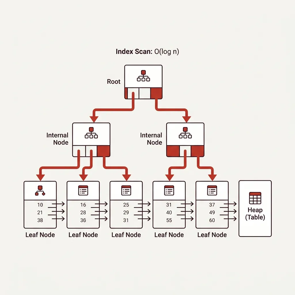
A B-tree is a balanced tree of sorted values. Here’s a simplified view of what an index on an email column looks like:
flowchart TD
    Root["Root Node\n[M ... T]"] --> Left["Internal Node\n[A ... L]"]
    Root --> Right["Internal Node\n[N ... Z]"]
    Left --> LL["Leaf Node\nadam@... | alice@... | bob@..."]
    Left --> LR["Leaf Node\ncharlie@... | david@... | emma@..."]
    Right --> RL["Leaf Node\nnick@... | oliver@... | paul@..."]
    Right --> RR["Leaf Node\ntom@... | victor@... | zoe@..."]

    style Root fill:#c0392b,color:#fff
Each leaf node stores the index key value alongside a heap pointer — the physical location of the full row on disk. When you search for customer@example.com, the database traverses the tree in O(log n) steps, finds the pointer, and fetches just that row.
For a table with 10 million rows, a B-tree index is typically 4-5 levels deep. Finding a value takes at most 5 page reads instead of hundreds of thousands. That’s the performance difference you see.
What “Balanced” Means and Why It Matters
The “B” in B-tree stands for balanced — the tree is always restructured to keep all leaf nodes at the same depth. This guarantees O(log n) worst-case access regardless of what values you insert or delete. It also means inserts and updates are more expensive, because the database may need to restructure the tree to maintain balance.
This is the first hint that indexes have a cost.
How the Query Planner Decides to Use an Index
Here’s something that surprises many developers: having an index on a column does not guarantee the database will use it.
The PostgreSQL query planner is a cost-based optimizer. It estimates the cost of different execution plans and picks the cheapest one. For each query, it weighs:
- The cost of a sequential scan (reading all rows, but sequentially from disk, which is fast)
- The cost of an index scan (random disk reads for each matched row, which is slow per-operation)
- The cost of an index-only scan (reading only from the index, no heap access)
- The estimated number of matching rows
The key insight: random I/O is more expensive than sequential I/O. On spinning disk, sequential reads are up to 100× faster than random reads. On SSDs, the gap narrows but doesn’t disappear.
So if your query is expected to match 30% of the table, a sequential scan might genuinely be faster than using the index — because reading 300,000 rows randomly from an index is slower than reading the same rows sequentially from the heap.
-- Check what the planner actually does
EXPLAIN ANALYZE
SELECT * FROM orders WHERE status = 'pending';
The output will tell you whether it used a sequential scan, an index scan, or a bitmap index scan. Learning to read EXPLAIN ANALYZE output is one of the highest-leverage skills in backend engineering.
The Types of Index Scans
PostgreSQL uses indexes in three different ways depending on the query:
Index Scan
The database walks the B-tree to find matching entries, then follows each heap pointer to fetch the full row. This is efficient for queries that match a small number of rows (high selectivity). For each matching row, it makes one random I/O to the heap.
Bitmap Index Scan
For queries that match more rows, PostgreSQL uses a two-phase approach:
- It reads the entire index for matching entries and builds an in-memory bitmap of which heap pages contain matching rows
- It reads those heap pages in page order (sequential-ish), rather than randomly
This is significantly more efficient for medium-selectivity queries. You’ll see Bitmap Heap Scan and Bitmap Index Scan in your explain plans.
Index-Only Scan
If every column your query needs is stored in the index itself, the database can answer the query without touching the heap at all.
-- If idx_orders_customer covers (customer_id, order_date), this may be index-only
SELECT customer_id, order_date FROM orders WHERE customer_id = 42;
Index-only scans are extremely fast because they eliminate all heap I/O. This is the foundation of covering indexes.
Composite Indexes: Column Order Matters
A composite index covers multiple columns. The critical rule: column order in the index definition determines which queries benefit from it.
CREATE INDEX idx_orders_customer_status ON orders (customer_id, status);This index helps:
- Queries filtering on
customer_idalone ✅ - Queries filtering on both
customer_idandstatus✅ - Queries sorting on
customer_idalone ✅
This index does not help:
- Queries filtering on
statusalone ❌ (can’t use the right side of the index without the left side)
flowchart LR
    Q1["WHERE customer_id = 42"] --> IDX["Index: (customer_id, status)"] --> FAST["Index Scan ✅"]
    Q2["WHERE status = 'pending'"] --> IDX
    IDX --> SLOW["Sequential Scan ❌\n(Index skipped)"]

    style FAST fill:#27ae60,color:#fff
    style SLOW fill:#c0392b,color:#fff
The general rule: put the most selective column first, and the column you filter equality on before the column you filter ranges on.
For a query like WHERE customer_id = 42 AND created_at > '2024-01-01', the index should be (customer_id, created_at) — equality condition first, range condition second.
Partial Indexes: Indexing a Subset of Rows
You don’t have to index all rows. A partial index only indexes rows that match a condition.
-- Only index rows where status is 'pending'
CREATE INDEX idx_orders_pending ON orders (created_at)
WHERE status = 'pending';
This is dramatically smaller than a full index on created_at if most orders are in a completed state. It’s also faster to update (fewer index entries to maintain) and more cache-friendly.
The canonical example: a jobs table with millions of completed jobs and thousands of pending jobs. A partial index on pending jobs means your queue worker queries hit a tiny, fast index instead of a massive one that covers historical data you never query.
The Write Cost You’re Paying
Every index is a separate data structure on disk. Every INSERT, UPDATE, or DELETE on a table must update every index on that table — potentially requiring B-tree rebalancing operations.
For a write-heavy table with 8 indexes, every insert is actually 9 writes (the heap + 8 indexes). Every update to an indexed column is at least 2 additional index operations (remove old entry, insert new entry).
-- Check all indexes on a table and their sizes
SELECT
    indexname,
    pg_size_pretty(pg_relation_size(indexrelid)) AS index_size
FROM pg_stat_user_indexes
WHERE relname = 'orders'
ORDER BY pg_relation_size(indexrelid) DESC;
If you have a table that receives 10,000 inserts per second and you add an index “just in case,” you’ve just added 10,000 extra write operations per second. At scale, this matters.
The discipline: index for queries you’re actually running, not queries you might run.
Hash Indexes
PostgreSQL also supports hash indexes. Unlike B-trees, hash indexes:
- Only support equality lookups (
=) - Do not support range queries, sorting, or pattern matching
- Are smaller than B-trees for the same data
- Are faster for equality lookups under the right conditions
CREATE INDEX idx_sessions_token ON sessions USING HASH (token);Use hash indexes when you only ever query a column with = and never with <, >, BETWEEN, or LIKE. Session tokens, API keys, and lookup codes are good candidates.
One important caveat: hash indexes were not WAL-logged before PostgreSQL 10, making them unsafe in replication setups on older versions. Always check your version.
Index Bloat
Over time, indexes accumulate dead entries from deleted and updated rows. PostgreSQL’s MVCC model means old row versions stay in the heap until vacuumed. The same applies to indexes — dead index entries accumulate until VACUUM cleans them up.
A heavily updated table with infrequent vacuuming will develop index bloat: an index that’s significantly larger than the data it indexes. This wastes disk space, wastes memory (index pages compete for the shared buffer cache), and makes index scans slower because there are more pages to traverse.
-- Check for index bloat (requires pgstattuple extension)
SELECT
    relname,
    pg_size_pretty(pg_relation_size(oid)) AS table_size,
    pg_size_pretty(pg_total_relation_size(oid) - pg_relation_size(oid)) AS index_size
FROM pg_class
WHERE relkind = 'r'
ORDER BY pg_total_relation_size(oid) DESC
LIMIT 20;
If your indexes are larger than your tables, something is wrong.
Practical Rules
After building and debugging production database systems, these are the rules we operate by at Ellomas:
1. Index foreign keys immediately.
Every foreign key column should have an index unless you’ve explicitly decided otherwise. JOINs on un-indexed foreign keys produce sequential scans on the child table. This is one of the most common causes of slow queries in applications with normalized schemas.
2. Measure before adding indexes.
Use EXPLAIN ANALYZE before and after. An index that looks like it should help might be ignored by the planner, or might cost more than it saves if the query isn’t selective enough.
3. Index your ORDER BY columns for paginated queries.
SELECT ... ORDER BY created_at DESC LIMIT 50 benefits enormously from an index on created_at. Without it, the database sorts all matching rows before applying the limit.
4. Consider covering indexes for hot read paths.
If a query is run millions of times per day and only selects 2-3 columns, make those columns the index. The index-only scan eliminates heap I/O entirely.
5. Drop indexes you don’t use.
PostgreSQL tracks index usage in pg_stat_user_indexes. An index with zero scans in the last month is pure overhead on your writes.
-- Find unused indexes
SELECT
    relname AS table_name,
    indexrelname AS index_name,
    idx_scan AS times_used
FROM pg_stat_user_indexes
WHERE idx_scan = 0
ORDER BY pg_relation_size(indexrelid) DESC;
Bringing It Together
Indexes are not magic. They’re a specific trade-off: spend more on writes and storage, gain on reads. The right index on the right column transforms a query. The wrong index on the wrong column silently taxes every write without benefiting any read.
The engineers who are best at this aren’t the ones who add the most indexes. They’re the ones who read query plans, understand their data distribution, and make deliberate decisions about what to index and what to leave as a sequential scan.
Build that habit. Run EXPLAIN ANALYZE on every slow query before you add anything. You’ll be surprised how often the answer isn’t “add an index” — and how much more powerful indexes become when you apply them selectively.
Ellomas Technologies builds reliable software for credit, power, and operations systems. We help teams design databases that perform under real load — not just under ideal conditions.